Power supplies
One often comes across a question like "what kind of power supply do I need?" The standard answer should be "that depends on your requirements, so find out what they are". There are, however, two types of power supply I find particularly useful in the electronics laboratory:
- Linear supplies (single and multiple output) with simple potentiometer adjustment, for experimental setups, functional testing and repair. Linear regulation and low output noise are required to avoid injection of unwanted signal components. Fanless models are preferred to avoid annoying fan noise during long sessions at the work bench. Models without a fan are unfortunately not that common, but a good starting point would be the E36xxA series from Agilent/Keysight.
- Programmable linear supplies, of high stability, for design characterization. Models with built-in current and voltage read-back facilities, such as the "dynamic measurement" DC sources from Agilent/Keysight, or the PM28xx series from Philips/Fluke, are highly useful, and may save external multimeters, depending on your accuracy requirements. As this kind of supply is often used for testing under software control and without the operator being present, a fan is acceptable.
|
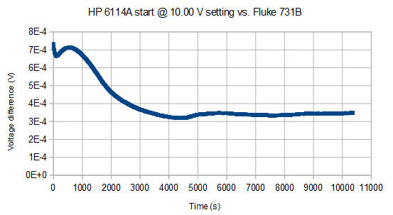
Hewlett Packard 6114A Precision Power Supply
The 6114A was presented in the HP Journal November 1972 issue and is still considered a reliable and stable power supply. Kudos to HP and the engineers! The 6114A and the sister model 6115A went through a couple of design changes, and one of latest versions, with seriel number prefix 3601A, is shown in the picture (to be inserted). The late versions feature a large rocker power switch, a 4-digit thumbweel voltage setting plus a single-turn potmeter for fine adjustment. Not also the hp logo without black/blue coloring, found only on the very latest models. The graph shows the voltage for the 6114A set to 10.00 V after power-on compared to Fluke 731B DC Reference Standard. The difference voltage was measured without load with a Fluke 8842A and the data was captured with LabVIEW. The voltage changes about 0.35 mV equal to 35 ppm over the first hour. Due to the stability, low noise, and lack of fan, the 6114A is perfectly suited for powering oscillators under test, and the current capacity of 2A below 20 V allows room for OCXOs with a high cold-state current draw. |
|
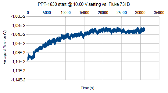
GW PPT-1830 GPIB
This is an example of a programmable power supply with a convenient form factor and 3 outputs for general purpose electronics design and test. A drawback of this particular model is the noisy fan, which runs at constant speed. The graph shows the voltage for the PPT-1830 set to 10.00 V without load after power-on compared to Fluke 731B. The voltage changes about 0.6 mV over the first 3 hours, which is quite well, but the fluctuations are significantly larger than those observed for the 6114A above. |
|
(Picture to be added)
|
Agilent 66312A Dynamic Measurement Source
The 66312A is an example of a highly stable single-output power supply with a valuable readback feature through GPIB. For setups requiring dual supplies, you obviously need two identical units, or to get a dual-output model with readback. The graph shows the voltage compared to the Fluke 731B reference, when the 66312A is set to 10 V. The lower graph shows the output voltage when pulsing with 1 A load at 0.1 Hz |
|
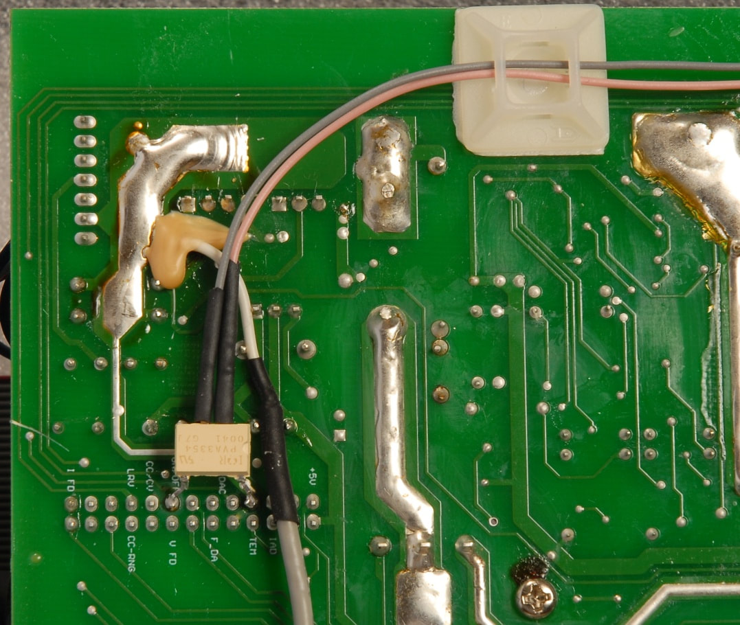
Adding control to the BK Precision 8540 DC Electronic Load
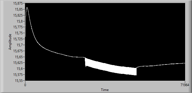
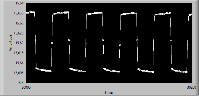
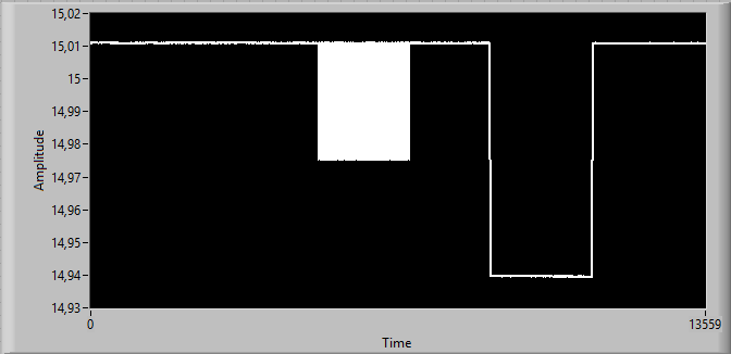
The 8540 is a handy electronic load in a practical form factor for testing your power supplies. The disadvantage is that it cannot be controlled from an external interface. However, there's a way of overriding the On/Off button so that the 8540 may be forced on by an external TTL signal: When pulling the node called ON/OFF to GND the 8540 turns on even if the On/Off button is set to Off. The picture shows how a PVA3354 LED to MOS optocoupler is used for this purpose. The LED is connected via a 330 Ohm resistor to an isolated BNC connector mounted on the back panel. When nothing is connected to this input, the 8540 then operates as normal. The switching rate is limited by the switching dynamics of the 8540, so observe the switching delay, and do not expect to switch faster than 1 Hz. Note also, that changes to the settings only come into force when you toggle the On/Off button. This means that you cannot change the load current while forcing the output active. Despite these limitations, the arrangement allows a very useful control to do simple automated tests. Finally, a word of caution: Should you get the urge to carry out such a modification, remember that it's at your own risk! As an example, the two graphs below the picture show the results from a test of an old Danica TPS1a power supply, using the control modification above. The first part of the upper graph shows the voltage from cold power-up. Then, after the unloaded voltage has settled, a pulsed load of 1 A with 4 s repetition period is applied. In the thrid part, the load is removed to let the supply cool. The lower graph is a close-up of some 20 s during the pulsed load. The voltage is measured with Fluke 8842A, at medium rate, which results in a sampling rate of close to 10 Hz. The voltage drop reveals an output impedance of the TPS1a close to 30 mOhms, which is lower than the specified 50 mOhms. The last picture shows a test of a GW PPT-1830 set to 15 V, with the load changing between 1 A pulsed and 2 A continuous. Note how the thermal effects of the load are much smaller in comparison with the old Danica TPS1a. Perhaps not a fair comparison, but it just demonstrates the value of dynamic testing of power supplies. |
|
Testing output impedance of power supplies
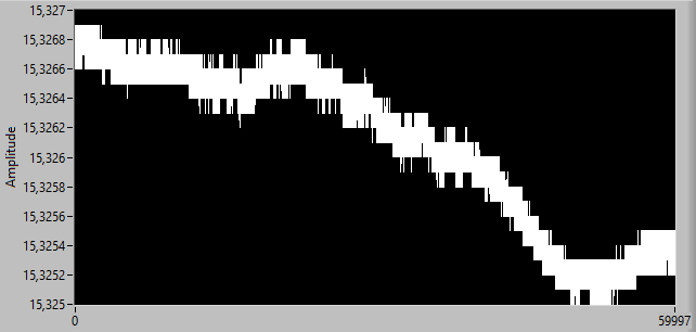
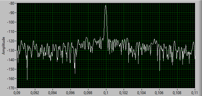
For low values of the output impedance, the measurement is carried out over a period of time and then an FFT is applied. The graph on the left shows the voltage over 60k measurements for an Agilent E3640A supply while pulsing with 500 mA, which is the maximum rated current for the 0-20 V outputs. The pulse period was 10 s, and cannot even be seen on the graph. The FFT, on the other hand, shows an amplitude of 98 µV at 0.1 Hz, thus an output impedance of merely 0.2 mΩ is found. |
