A look at RMS measurements
Being able to measure RMS correctly plays a particular role when it comes to AC level measurements. Typical applications include power supply characterization, amplifier noise measurements, weighted audio measurements, etc. Important parameters to look for are the bandwidth at different levels, the measurement accuracy and stability, the linearity over a range, and the noise floor. Other topics of interest could be data interfaces, measurement speed, user-selected bandwidths, the ability to show results in a dB scale, a choice between an analog or digital readout, or perhaps to have both. Some RMS voltmeters include DC measurements, but a multimeter is a better choice for that specific purpose, I believe. The important feature of RMS voltmeters is that they measure the RMS of AC signals, and that they carry out this task well. Don't forget, by the way, when absolute level accuracy is called for, you need to calibrate your AC measurement gear. I use the Fluke 510A AC Reference Standard in combination with an inductive voltage divider for in-house calibration.
I have compiled this overview out of my interest in RMS measurements, and in order to help others to find out which voltmeter to put in work for a task. I hope you find it helpful. If you have comments or questions, leave a not on the contact page.
I have compiled this overview out of my interest in RMS measurements, and in order to help others to find out which voltmeter to put in work for a task. I hope you find it helpful. If you have comments or questions, leave a not on the contact page.
|
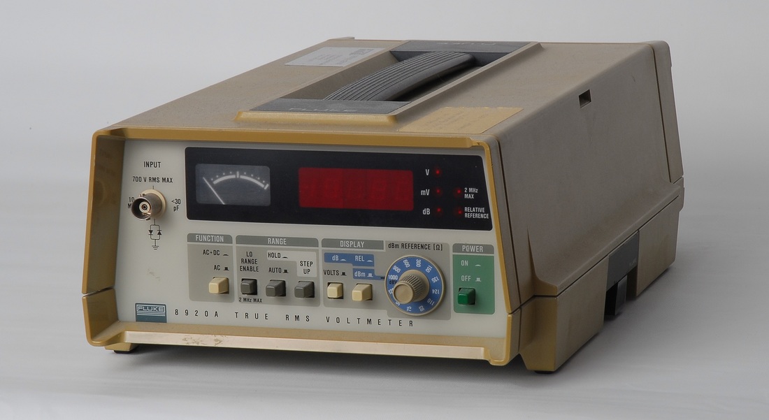
Fluke 8920A True RMS Voltmeter
The detector in this voltmeter uses a pair of thermally isolated resistor/transistor elements (Fluke part 489377) where the AC power and DC power in each of the two resistors are made equal by using the transistor pair as the heat difference sensor. Golden area: 50 Hz - 200 kHz and 18 mV - 700 V for 0.5 % AC accuracy, up to 20 MHz for 5 % accuracy. With its digital readout, the autorange feature and the impedance reference settings I generally favour the 8920A over the HP 3400A. The bandwidth of the 8920A is limited to 2 MHz in the 2 mV range, however, so noise measurements of power supplies requiring 20 MHz bandwidth will have to be done in the 20 mV range, though accuracy at low levels becomes an issue. Ideally, a low-noise, wideband amplifier with +20 dB gain in front of the 8920A should be used for such measurements. |
|
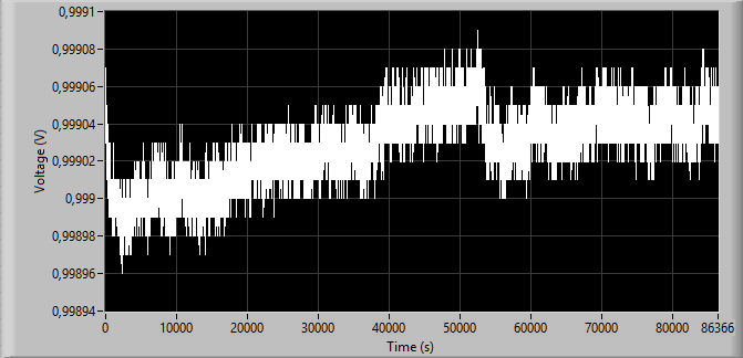
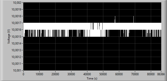
The graph shows the voltage on the output on the back of the 8920A over 24 hours for a 10 V signal at 2.4 kHz from the Fluke 510A (1 V DC equals 10 V AC RMS). The DC voltage was measured with a Fluke 8842A using external triggering. Note how the changes during warm-up are small and comparable to the changes over a 24 h period. The relative standard deviation for the last 20 hours (duration chosen to compare with other RMS instruments below) the relative standard deviation is 15.6 ppm .
|
|
|
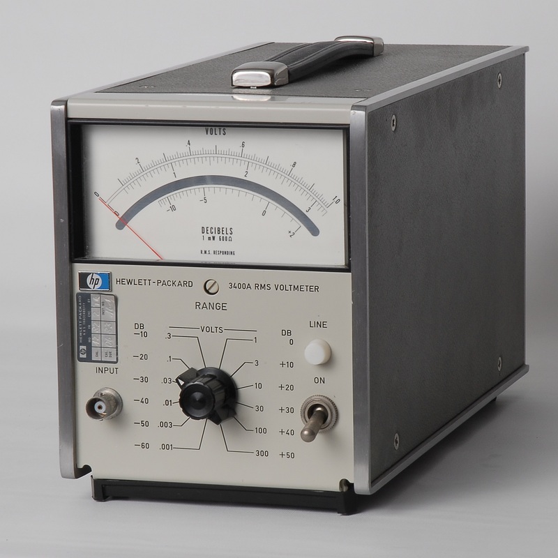
HP 3400A RMS Voltmeter
In this classic instrument a chopper amplifier balances the voltage generated by two thermocouples so that the AC power applied to one of the thermocouples corresponds to the DC power applied to the other. Golden range: 50 Hz - 1 MHz for 1% of full scale, up to 10 MHz at 5 %. Note that older versions of the 3400A use a cathode follower in the input and a photochopper amplifier, while newer versions use a FET in the input and the ICL7650S chopper-stabilized OP-AMP. The upgraded 3400B had an extended frequency range up to 20 MHz. |
|
The graph shows the voltage on the output on the back of the 3400A over 24 hours for a 10 V signal at 2.4 kHz from the Fluke 510A (-1 V DC equals 10 V AC RMS). The DC voltage was measured with the Fluke 8842A using external triggering.
The 3400A manual states that one should wait 5 minutes for the 3400A to warm up before making a reading, or 30 minutes before making performance checks. However, based on the results shown here, the warm-up period more likely seems to be around 2 - 3 hours if you want to get the full accuracy of the DC-output. Note also how the readings of the 3400A are relatively noisy, resulting in a relative standard deviation of about 124 ppm over the last 20 hours. |
|
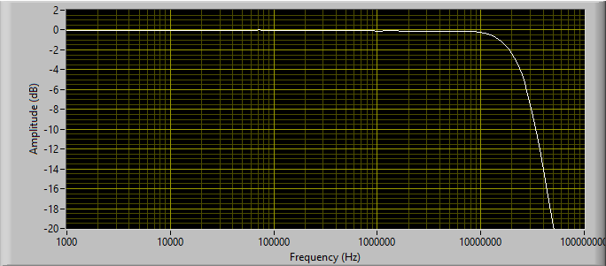
The graph shows why the old 3400A still is an interesting piece of measurement gear. The bandwidth extends to 10 MHz even in the 1 mV range, and is 3 dB down at about 23.5 MHz.
The sweep from 1 kHz through 100 MHz was made using an 3577B as source and level monitor, while acquiring the DC-level on the back of the 3400A with a Fluke 8842A multimeter. |

Picture to be uploaded
|
HP 3586C Selective Level Meter
The instrument was marketed exclusively as a selective level meter, but actually has a valuable wideband RMS measuring feature. Furthermore, the bandwidth is preserved at low levels. When operating in its wide-band mode the 3586C uses incoherent downsampling to generate a signal that has a reduced bandwidth but a representative RMS level. A diode bridge samples the input signal, and an AD536 (absolute value plus squarer/divider circuit) converts the sampled signal to DC which then is digitized. A neat solution though the accuracy will depend on the crest factor due to the AD536. The specified frequency range of the wideband mode is 200 Hz to 32.5 MHz, over -45 dBm to +20 dBm. The golden range is 20 kHz - 10 MHz for 1 dB accuracy, while 2 dB accuracy is specified for 200 Hz - 32.5 MHz. |
|
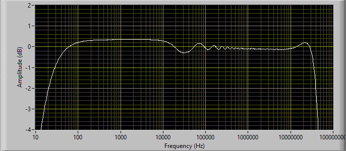
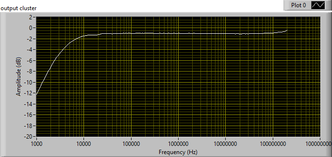
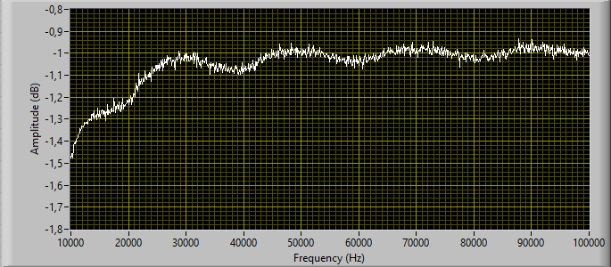
The measurements here shows how the 3586C wideband response stays within 1 dB between 33 Hz and 34 MHz, and is within 3 dB between 17 Hz and 42 MHz. This makes the 3586C a candidate for power supply noise measurements, but keep one thing in mind: The input of the 3586C is DC-coupled, so you need a proper protection network with AC-coupling before you even think of applying DC to the input.
The graph shows the response, made at 1 mV RMS input level. With a 50 Ohm source the 3586C display shows a noise floor of -95 dBV (18 µV), which is quite well considering the close to 42 MHz noise bandwidth. The incoherent sampling in the 3586C is implemented with a swept VCO as sampling generator, much in line with the 3406A, though the frequencies involved are different: 80 Hz FM of a 20 kHz - 50 kHz VCO in the 3586C, but 10 Hz FM of a 10 kHz - 20 kHz VCO in the 3406A. As a result of the specific implementation, there's some ripple of the frequency response, about 0.5 dBpp, which is significantly more than the 0.1 dBpp for the older 3406A. |
|
Picture to be uploaded
|
Sennheiser Universal - Pegelmessgerät UPM 550-1
The instrument targets audio measurements with its various weighting filters, and the working frequency range in the RMS mode is limited to 10 Hz - 100 kHz. A bulit-in pre-amplifier allows measurements at low levels. The AD536 takes care of the RMS-to-DC conversion, so the accuracy will depend on the frequency, level and crest factor. You should consult the AD536 datasheet for better understanding your UPM 550-1. |
|
Picture to be uploaded
|
Fluke 8506A Thermal RMS Digital Multimeter
Just like the Fluke 8920A True RMS Voltmeter the Fluke 8506A Multimeter uses a pair of thermally isolated resistor/transistor elements for the RMS-to-DC conversion, though it's a different Fluke part 521625 for the 8506A. The 8506A applies an iterative computation to enhance the accuracy. Best range: 40 Hz - 20 kHz with 0.012% of reading in the high accuracy mode over 24 hours excluding aging. Up to 1 MHz with 3.5 % accuracy. |
|
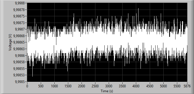
The graph shows the measured AC voltage by the Fluke 8506A with the Fluke 510A (2.4 kHz) as the source over 12 hours, after 12 hours of warm-up. Results were captured through GPIB using LabVIEW.
The settings of the 8506A were VAC Hi Accuracy with Filter and Avg enabled. As a result, the measuring rate is rather low, with some 7.35 s between results, but the relative standard deviation is 3.30 ppm. |
|
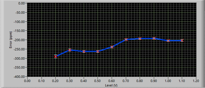
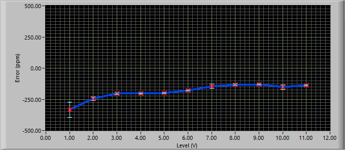
The graphs show a test of the accuracy and the linearity for the 12.5 V and the 1.25 V AC ranges of the Fluke 8506A. The source was a Fluke 510A at 2.4 kHz via an inductive voltage divider ESI DT72A. The settings were VAC Hi Accuracy with Filter enabled. The error bars are a measure of the standard deviation observed over 32 measurements.
The 8506A could do with an adjustment, but I'd rather have a knowledge of the correction factor in each of the ranges. |
|
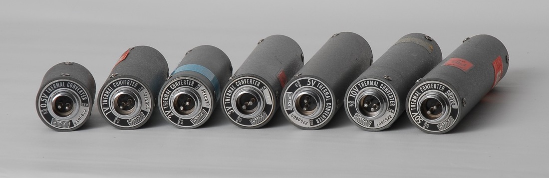
Fluke A55 Thermal Converters
The A55 series of thermocouples target different operational voltages for AC level metrology. They are to be used together with a low-level DMM or in a bridge configuration with a DC source and a difference voltmeter. I use the Keithley 181 Nanovoltmeter as it provides 10 nV resolution in its 20 mV range with < 30 nVpp noise. Great care should be exercized in order not to overload the thermocouple! Watch out for level transients when switching range of a generator, for instance! A variety of converters (in my case 0.5, 1, 2, 3, 5, 10 and 50 V) allows calibration of different sources. |
|
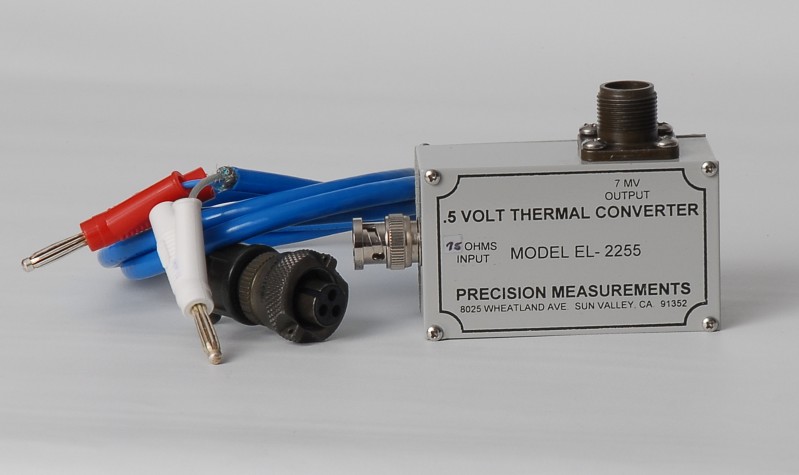
Precision Measurements EL-2255 Thermal Converter
This specific thermocouple is dedicated to 75 Ohm systems for level calibration about 0.5 V RMS, but the EL models are available for different levels and impedances. Again, a low-level voltmeter, such as the Keithley 181 Nanovoltmeter, can be used for measuring the DC voltage. |
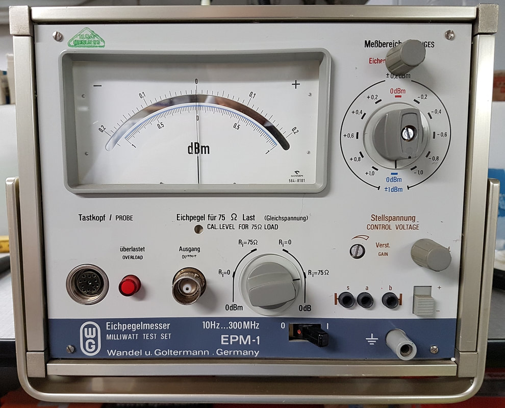
The EPM-1, here shown without test probe connected. Note the DC calibration output "Ausgang" with the 3-lug type 1.6/10 connector.
Above: The unbalanced test probe TK-10 for the EPM-1, here in a 75 Ohm version. (Picture to be added)
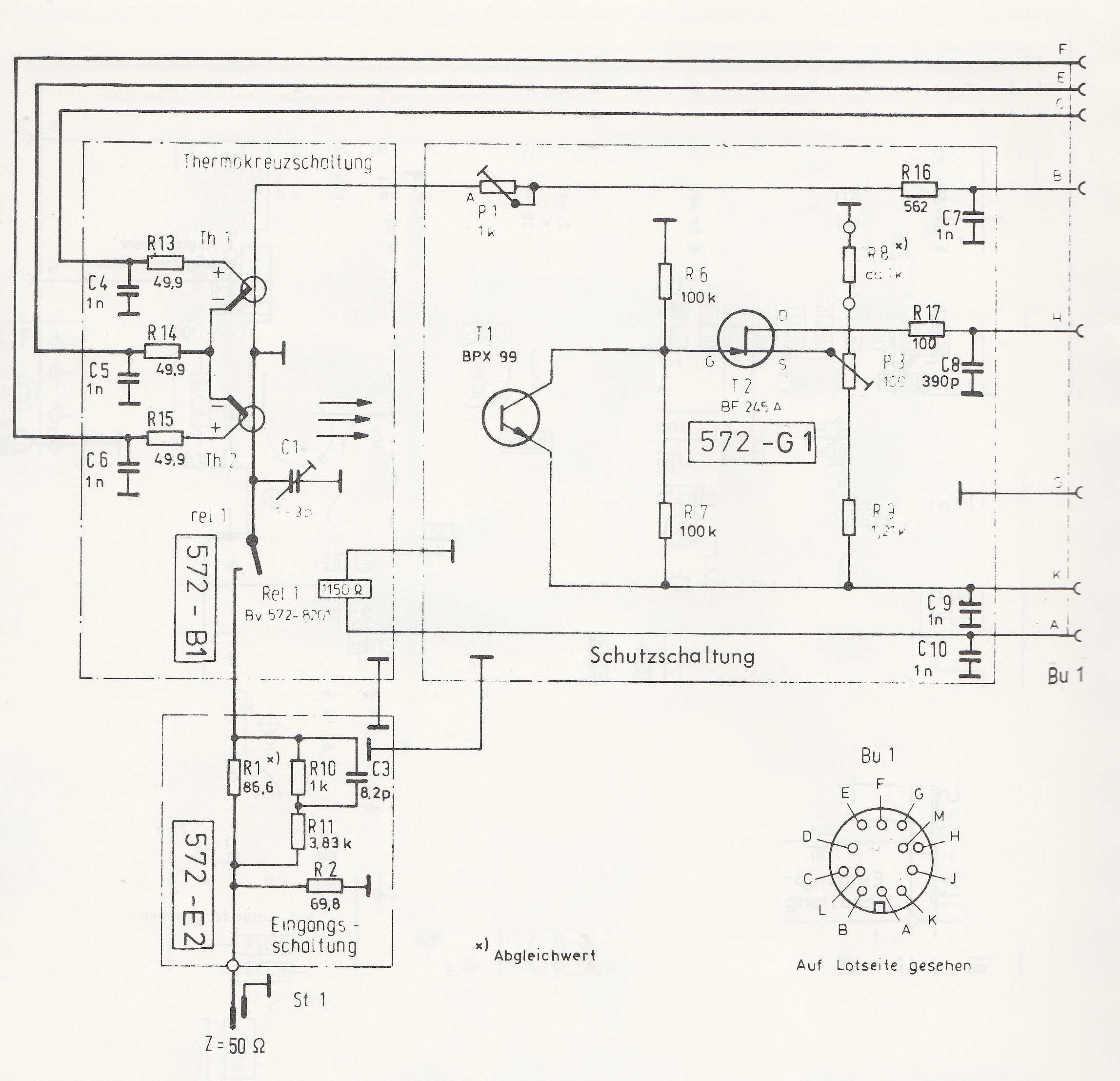
Schematic detail of the TK-10 probe with the two thermocouples, scanned from the EPM-1 manual. In the 75 Ohm version R1 is replaced with 84.5 ohm, and R2 with 130 Ohm.
|
Wandel & Goltermann EPM-1 Milliwatt Power Meter
So here's an interesting piece of equipment, dating back to around 1970. The EPM-1 targets specifically the measurement of power close to 0 dBm, but does this quite well. The wide frequency range between 10 Hz and 300 MHz is hard to beat, and the accuracy at 0 dBm at the test probe input is stated to ±0.015 dB up to 50 MHz, and ±0.05 dB up to 300 MHz. Care is required by the user not to ruin the accuracy by loss and mismatch in cables and adaptors. With proper consideration of these effects, the EPM-1 may serve as an RF level calibrator, even today, half a century later after its introduction... The EPM-1 is based on two thermocouples, one for the input, and another for a DC feedback. The two thermocouples are brought in balance through a chopper amplifier and a synchronous detector. For slight overloads (above approx. 1.7 V) the EPM-1 includes a mechanism to protect the input thermocouple, but one should never apply more than 3 V AC or DC to the input as this will almost certainly destroy the thermocouple. Hence, the protection is only useful in a very narrow power range, so treat the test probe with care! One annoying thing about the EPM-1 is the use of the 3-lug type 1.6/10 (IEC 75-7) connectors for the 75 Ohm version. The 50 Ohm version of the EPM-1 (which seems to be quite rare!) uses N-connectors. In the EPM-1 manual Wandel & Goltermann even argue why they went for the type 1.6/10 connector. In order to put the EPM-1 into use 1.6/10 adaptors are required, and the errors introduced should be accounted for. In addition to the unbalanced test probe TK-10, in the 50 Ohm or 75 Ohm version, W&G also offered a balanced version, the TKS-10, to be used with one of their balanced impedance adaptors for 124 Ohm, 150 Ohm or 600 Ohm environments. In addition to the test probes W&G also provided a T-splitter, attenuators, and a range of adaptors for the 3-lug 1.6/10 connector and for the N connector. |
|
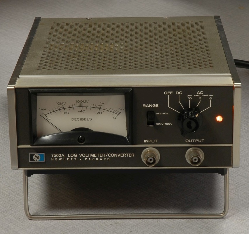
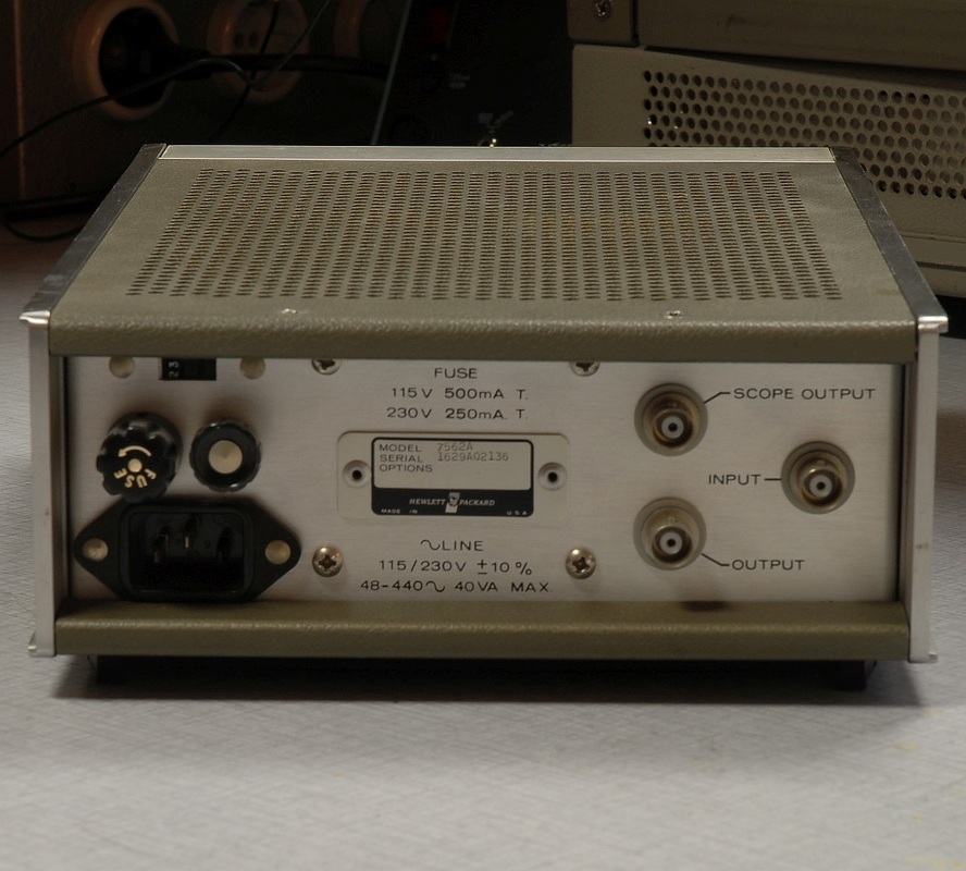
HP 7562A Log Voltmeter / Converter
The 7562A uses a thermocouple with an electronic attenuator between the pre-amp and the thermocouple driver. The attenuator design includes matched FETs in combination with a DC control loop to linearize the attenuator. This makes it possible for the 7562A to span 80 dB without changing range setting. A note on thermocouples: I once purchased a defective 7562A where the previous owner had tried to install an alternative thermocouple, most likely because the original thermocouple had been damaged somehow (despite of the protection mechanism). However, the attempt was bound to fail due to diverging thermocouple specifications. I was lucky to get a new (old stock) 0853-0007 thermocouple from a dealer and managed to calibrate the 7562A. BTW: The service manual is a MUST if you plan to fiddle with the 7562A, such as making adjustments! |
|
|
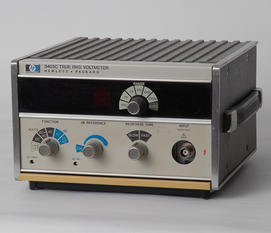
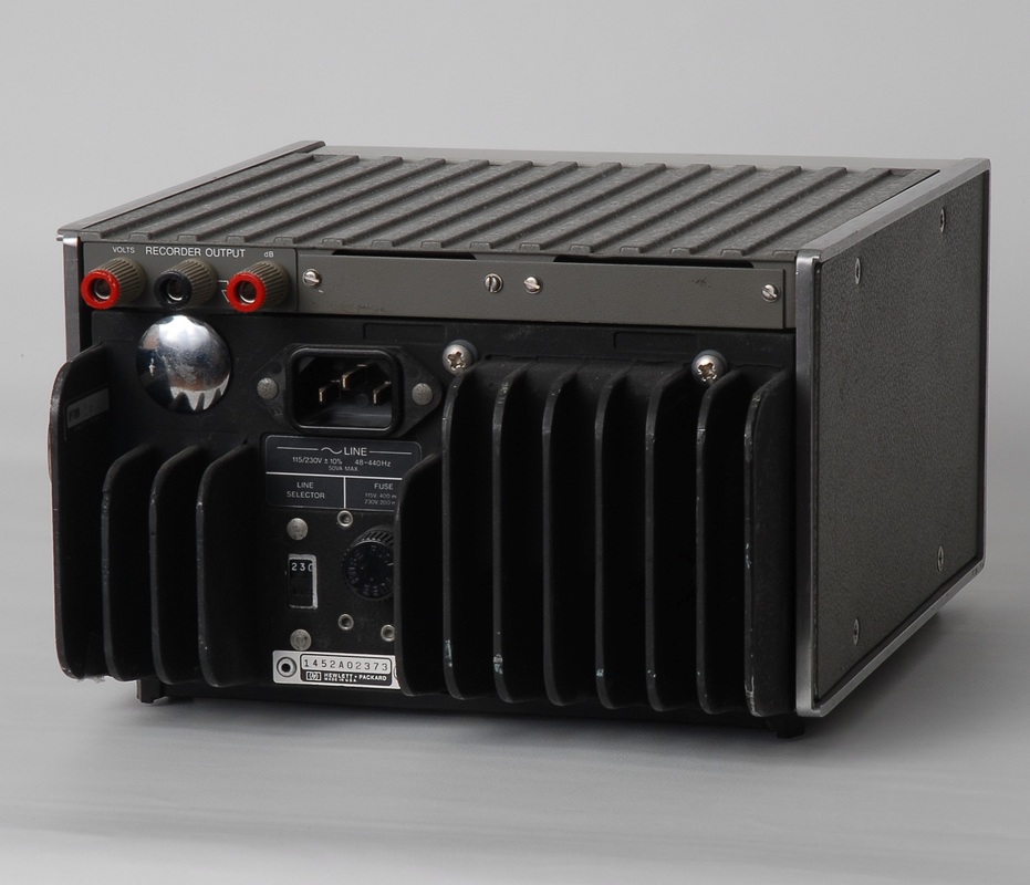
HP 3403C True RMS Voltmeter
This is another AC/DC thermocouple design, basically like 3400A. However, there are some important differences. The 3403C uses a multi-junction thermopile, with a quicker response than the thermocouple in the 3400A. The 3403C has also a wider frequency range, from 2 Hz and up to 100 MHz, and max. level up to 1 kV. The bandwidth is limited to 2 MHz in the 10 mV range, however, which is a clear drawback compared to the 3400A or 3400B. The bandwidth limitation prevents the 3403C from being used for power supply noise measurements often calling for 10 or 20 MHz bandwidth, often at 1 mV sensitivity. The unit shown on the pictures features autoranging (option 001) and dB scale (option 006). |
|
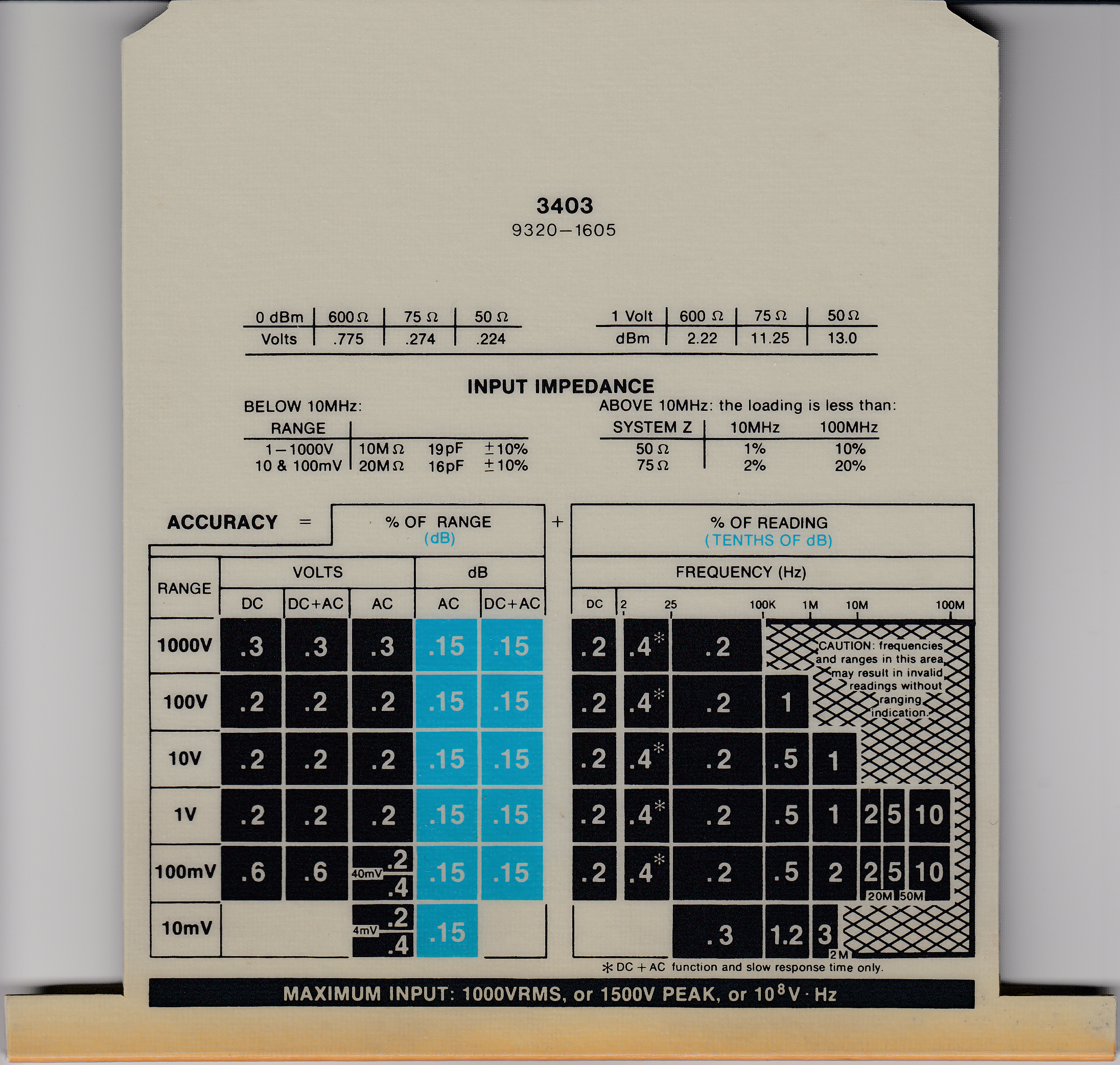
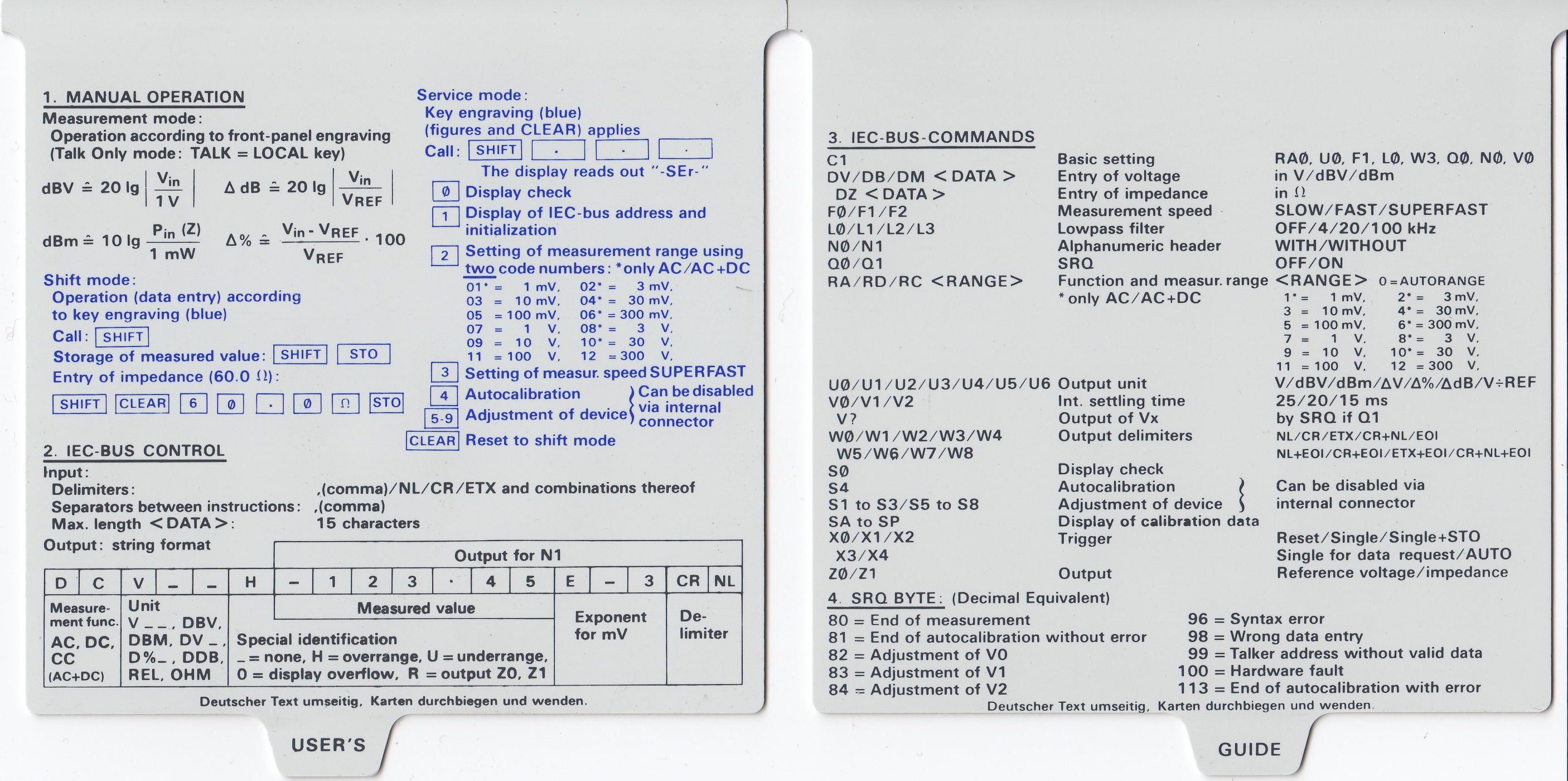
The specification card (HP part no. 9320-1605) is often in a miserable condition for the units that are put up for sale. Should you need to replace the card with a laminated print, for instance, the scan to the left can be used.
The width of the card is 146 mm (though 185 mm by the front), and the length is about 176 mm. if you want the card to bend as the original card in plastic you need to extend the length of you copy with about 6 mm. Another solution could be to glue an L-profile in plastic in front on the laminated copy. Mind you, however, that I have tried none of this as the card of my 3403C is in fine condition (as should be clear from the scan....) Click on the picture, and you will get a .png file having an appropriate resolution. |
|
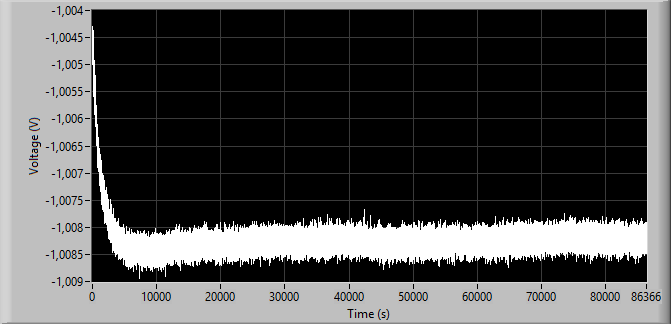
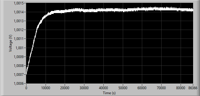
The graph shows the voltage on the output on the back of the 3403C over 24 hours for a 10 V signal at 2.4 kHz from the Fluke 510A (1 V DC equals 10 V AC RMS). The DC voltage was measured with a Fluke 8842A using external triggering. After some 4 hours the readings have stabilized. For the last 20 hours the relative standard deviation is 10.6 ppm. Once the 3403C has heated up, it appears more stable than the Fluke 8920A.
The 3403C manual recommends 15 min. warm-up before carrying out measurements, "sufficient warm-up" before proceeding with performance checks, and 1 hour warm-up before carrying out adjustments. In view of the above, I would go for a warm-up period of 4 hours. |
|
|
|
Fluke 8842A with Option –09 True RMS AC
An example of a classic 5½ digit multimeter, the Fluke 8842A from about 1990, with RMS capability. The option -09 adds an RMS module where an IC (Fluke stock no. 841900) takes care of the RMS to DC conversion. By using the traditional squaring, division and filtering approach, performance is only modest in terms of crest factor, frequency span, etc. |
|
(Images to be uploaded)
|
|
The graph shows the readings from the 8842A measuring a 10 V signal at 2.4 kHz from the Fluke 510A over 24 hours. The 8842A was heated up for 48 hours before the measurement. The relative standard deviation is 4.06 ppm, which seems quite well in view of the conversion principle.
|
|
HP 3406A Broadband Sampling Voltmeter with external RMS meter
This is an interesting combination if you need to do wideband RMS measurements. The 3406A uses incoherent sampling and provides an output of the sampled signal on the back panel. Connect this output to an ordinary RMS meter, and you may now carry out RMS measurements over a bandwidth determined by the 3406A. The graph shows the response using the 3577B as source and level reference. The Fluke 8842A measured the AC level on the Sample Hold Output on the back of the 3406A. In the graph the probe was connected directly to the Probe-to-BNC adapter, without the Isolator Tip (11072A). Note that the graph is offset with about 1 dB as no actual level calibration was carried out during this response test. The graph shows the response for a 10 mV signal, but the response for 1 mV is very similar. There's a few issues to keep in mind should you want to try to put the 3406A into use as a broadband RMS meter: A) The LF cut-off frequency of the 3406A is relatively high, so the combination is not directly suitable for measuring power supply ripple and noise. You may, however, split up the signal so that the 3406A measures the high frequencies, while another device measures the low frequencies. B) The sampling probe is inherently susceptible to overload and will be destroyed by too high an input voltage. Be sure to insert proper protection between the probe and item under test. Connecting the probe to an energized power supply, or switching a supply on/off while the probe is connected to it may burn out the probe. C) The gain from the probe tip to the sampling output is not well defined, though it nominally should produce 316 mV at full scale deviation. You need to calibrate the setup using a source with a known level before taking measurements. D) The sampling is not really random but the sampling frequency merely varies between 10 and 20 kHz at about a 10 Hz rate. For that reason, a slight ripple of the response can be seen, particular below 100 kHz, as shown on the lower figure on the left. E) At the lowest ranges (1 and 3 mV) you need to compensate for the noise floor of the 3406A to improve the accuracy. F) Finally, and that's an annoying thing about the 3406A: The push buttons for the range setting are not very reliable, so keep the contacts clean and do a sanity check of the level! |
|
(Image to be uploaded)
|
Hewlett Packard 438A power meter + 848x sensors
RF power meters are the answer if bandwidth rather than dynamic range is what you are looking for. Finding a second-hand power meter is no issue. They are available in large numbers at very low prices. More patience is required to find a power meter with a power sensor and cable, or sensors sold individually, at a reasonable price. From a company close-down years back I was lucky to get a set of 435A and 435B power meters with two 11730A cables, and 4 sensors, two 8482A, a 8483A and a 8481A, all for free! The 435A and 435B were later replaced with a 438A, shown in the picture, to create test setups under GPIB control. A dual-channel power meter like the 438A has the advantage that it may double as a scalar network analyzer; Add an RF generator and a splitter and run the meter and generator under GPIB control, and you got a network analyzer with a favourable form factor. |
|
(Image of the 323 to be uploaded)
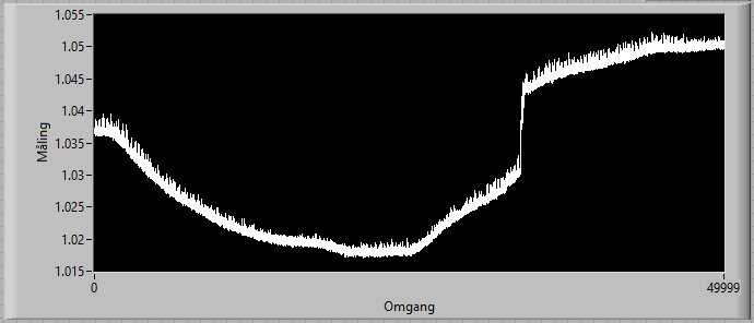
The output of the Ballantine 323 measured for a 1 V source over 50,000 s shows some substantial variations, though the 323 had been warmed up for hours in advance. The signal source was a Fluke 510A (2.4 kHz) in combination with a Gertsch RT-60 inductive voltage divider.
The temperature of the top of the enclosure was measured while acquiring the output voltage: The temperature at the start was 29.69 C, in the flat part of the curve in the middle the temperature was 28.81 C, and the temperature at the end was 29.63 C. The resulting temperature coefficient, based on the change from the start of the graph to the flat part, is 0.67 %/°C, with squareroot applied to the measured voltage. This is far worse than the typical 0.1 %/°C specified by Ballantine. The jump is not really explained for, but one probable cause could be an unreliable range switch. |
Ballantine 323 True RMS AC voltmeter
The model 323 from Ballantine has been around for decades, and has undergone a number of changes since its introduction. The first versions were based on two "uni-tunnel" diodes type HU5A in combination with a mechanical chopper and an AC-amplifier. This was later replaced with two schottky diodes followed by ICL7650 chopper amplifiers. In both cases the diodes run at low voltages so that they remain inside the square region (voltage proportional to power). There's no square root function built into the instrument, so the DC output on the instrument's back panel provides a voltage proportional to power. The advantage of the instrument is that the scale of the meter is linear in dB, and you may modify the filter to get a faster response than most other bench meters. I found, however, a few drawbacks of the instrument: 1) The BNC connector and the terminals on the front panel are located so that they are difficult to access, 2) The thermal drift is quite large, 3) The instrument is very susceptible to RF interference. Hopefully Ballantine have improved the models currently being marketed. Finally, once you need to adjust the instrument, you have to go through a rather cumbersome procedure which requires that you remove different parts of the enclosure. The unit purchased from the well-known fleabay market was described by the seller as "in good condition, tested and working". However, once it arrived, it was soon clear that it was not working properly at all, and had even been tampered with: Screws were missing, the knob for the functional switch was positioned wrongly, and the unit was plagued by a huge and varying offset. Clearly, someone in the past had tried to repair the meter and had given up. Given the fair condition of the unit, and my interest in seeing how it would perform in comparison to other RMS meters, I decided to repair it. Details on the repair are shown in the repair section. |
|
(Image to be uploaded)
|
NI USB-4431
With a maximum sampling frequency of 102.4 kHz the USB-4431 will not be put into use for measuring wideband noise from power supplies or anything similar. The advantages of the USB-4431 are its 24-bit resolution, its flexibility with the four input channels and one output channel, and its integration into LabVIEW and the powerful signal processing routines. The graph on the right shows a measurement of a 1 V signal from the Fluke 510A (2.4 kHz) through an inductive voltage divider, the Gertsch RT-60. LabVIEW's RMS-measuring VI was used, with 100 kHz sampling and 100 kS to provide a reading once per second. |
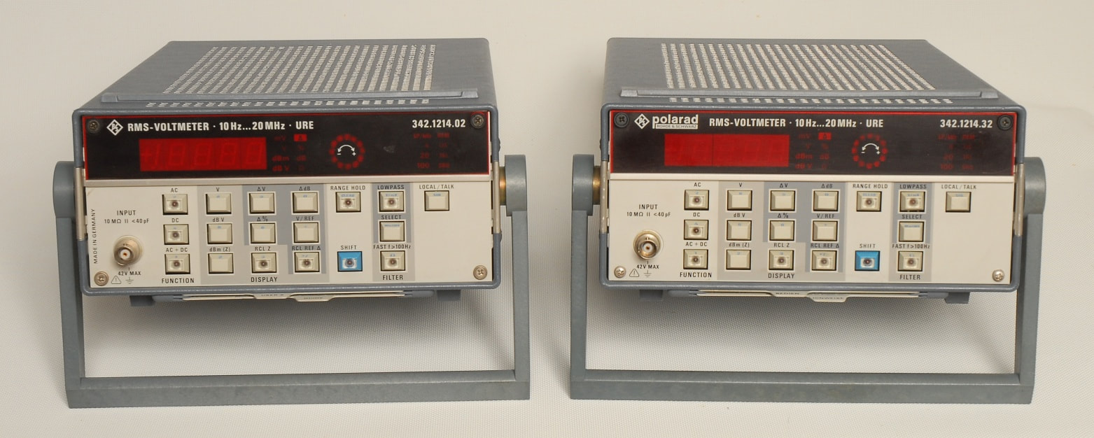
The URE in Rohde & Schwarz and in Polarad disguise.
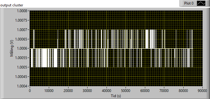
The URE is quite stable, as demonstrated by the above measurement over almost 24 hours of 1 V RMS, provided by a Fluke 510A via a Gertsch RT-60 inductive voltage divider. It appears that the URE could have benefitted from having one additional digit of resolution.
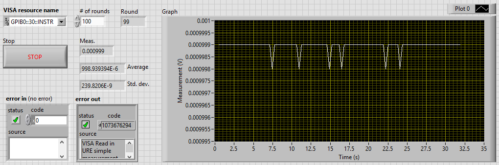
The measurement data were acquired through the IEC625 interface by a LabVIEW application. Note that the LabVIEW library available from Rohde & Schwarz for the more recent URE3 cannot be used for the URE due to the huge differences between the two products' programming syntax. The description of the programming URE manual is not very clear, so below is a LabVIEW snippet and its front panel to get you going. Just click on the pictures for full resolution. The snippet has no capabilities to set up the URE, so you need to set up the URE manually. Once started, the snippet merely queries the measurements a number of times. The snippet was used for the measurement over 24 h above. 
|
Rohde & Schwarz / Polarad URE RMS Voltmeter
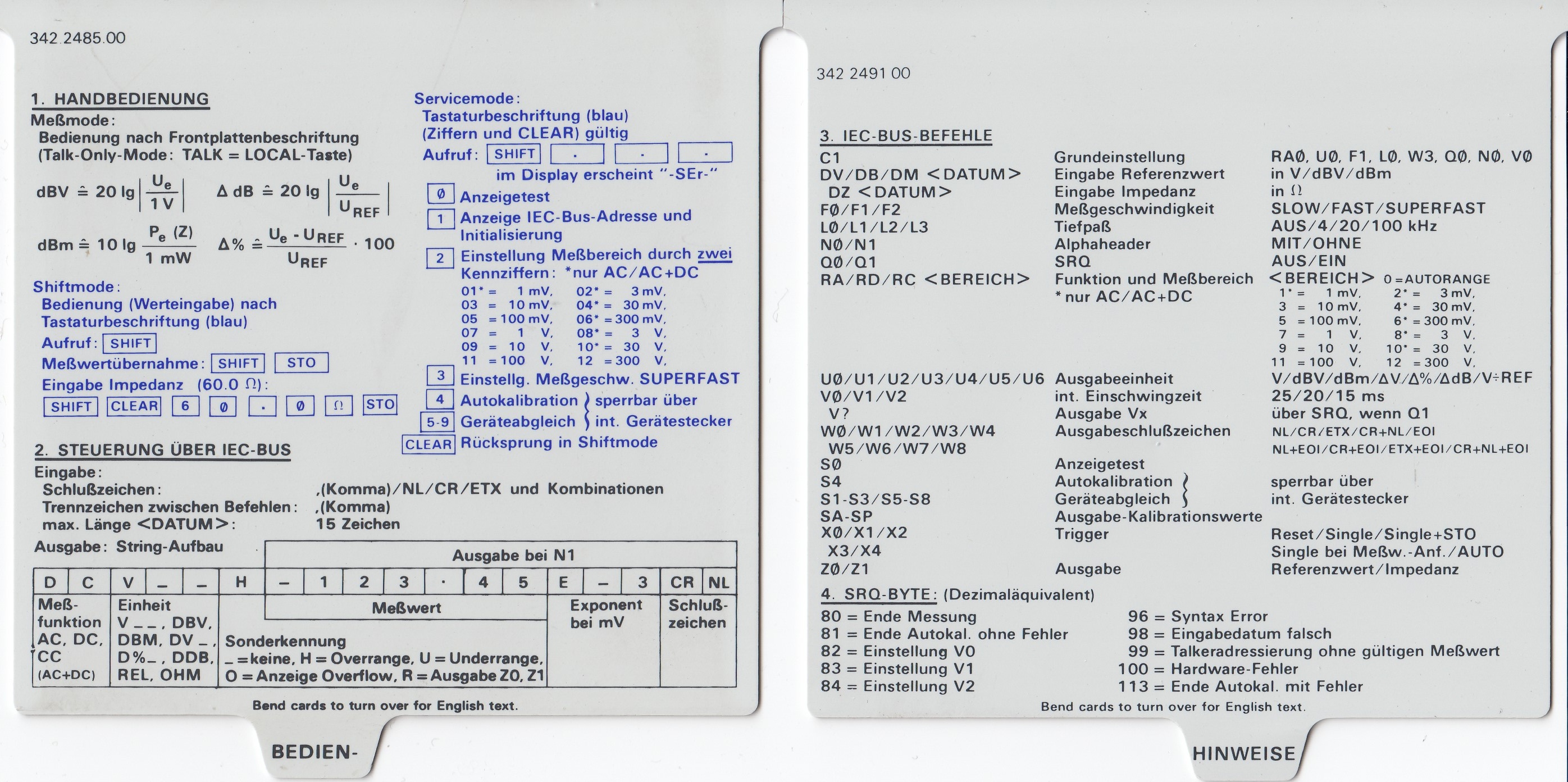
The URE, branded as either Rohde & Schwarz or Polarad, utilizes the non-linearity of a dual N-channel JFET for detecting the RMS voltage. The FET in question is listed as a "Siliconix WD115-SEL.AUS-U251" in the service manual. The description suggests that a WD115 is perhaps a selected U251. The criteria for the selection remain a secret in the URE service manual, but the pinch-off voltage is stated to be somewhere between 1 and 1.5 V. The URE features a two-tier self-adjustment routine based on an injection of known signals: The first step, called the "autocalibration" must be invoked by the user after repair or when the back-up battery has been replaced. This "autocalibration" targets the parameters that are considered time-invariant, such as divider ratios, and one constant in the used expression for the JFET characteristics. The second step, called the "rectifier calibration", is carried out automatically at regular intervals during a measurement and targets two JFET parameters that change with time and temperature. The URE features a DC output as option B2, but don't bother looking for it: The output is driven by a 12-bit A/D-converter, and provides thereby lower resolution than the actual measurement. Of value is the option B1, an IEC625-bus (labelled IEEE 488 on the Polarad models) to allow remote control and transfer of measurement results. The details of repairing three DOA units are shown in the repair section. The inserts with a short description in English and German of the operation are sometimes missing, so I've made scans that you may use to print out on paper and laminate. Just click on the pictures to access a copy with a high resolution. The inserts are 112 mm wide, across the area with the text.
|
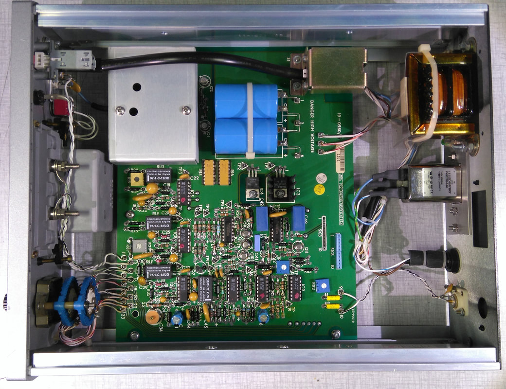
The inside of the Racal-Dana 9300B.
The build of the 9300B is very neat. The four photos were taken with the screening lid removed to show the input attenuator and the FET buffer circuitry. The IEC power inlet is not the original, and the 9300B was wired for 240 VAC only by the previous owner.
|
Racal-Dana 9300B RMS Voltmeter
The 9300B is as simple as can be: A power switch, and a range setting. There's no autoranging, and the instrument measures AC only. An additional feature is the switch which allows to either isolate or join the power and signal grounds. The benefit of the 9300B is the wide bandwidth, also at the most sensitive ranges. The design is based on a differential multiplier with integrator, plus remedies for noise and offset cancellation. A thorough description is found in the maintenance manual of the 9300 RMS Voltmeter, available on the Internet. A nice design feature of the range setting is that the rotary switch on the front panel does not handle signals directly. Instead, it switches a number of relays in the chain of attenuators and amplifiers. The models 9300 and 9300B have a different casing, but the schematics of the 9300 seem to apply to the 9300B, with a slight difference: In the 9300 a number of 1 % and 0.1 % resistors determine the gain and attenuation. In the 9300B, only 0.1 % resistors are used for this purpose. Still, it's interesting to learn that the R14 at the output of the FET buffer is a 5 % carbon resistor, and changes of this resistor will change the overall gain as it takes part of the first half of the 40 dB attenuator. I replaced the R14 with a metal film resistor, and as a result, the 9300B now appears more stable. 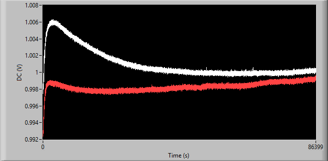
The graph shows the changes of the rear DC output over a period of 24 hours starting from power-up. The source was 1 V RMS from Fluke 510A via an RT-60 inductive voltage divider: With the original R14 carbon resistor (white), and with R14 replaced with a metal film resistor (red). The standard deviation is about 3 times lower with the metal film resistor.
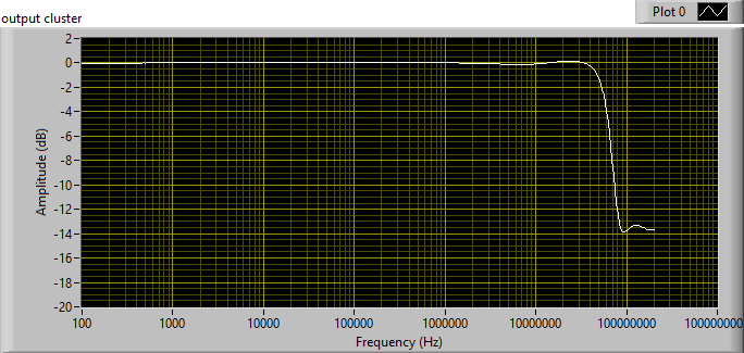
The 9300B excels with its wide bandwidth, demonstrated by the figure here which shows the response for 1 mV RMS input. The 9300B is 3 dB down at around 57 MHz, which makes it one of the candidates you could use for measuring wideband noise from power supplies, for instance. For power supply tests requiring an RMS meter with 10 MHz or 20 MHz bandwidth the 9300B is one of the RMS voltmeters where bandwidth reduction by means of a suitable lowpass filter should be considered.
|


|
Picture to be added: Stability of the DC output when measuring 10 V @ 2400 Hz from a Fluke 510A.
Picture to be added: Transfer function from RMS to DC level on the back panel, while staying in the same 2 V range. The level is set by an inductive voltage divider sourced by the Fluke 510A.
|
Marconi Instruments 2610 True RMS Voltmeter
Similar to the Fluke 8920A the Marconi 2610 is based on an NPN transistor pair where each NPN transistor is heated by a resistor, one for the signal being measured, and another for the DC signal to balance the transistor pair, thereby representing the RMS value. The NPN/resistor circuit in the 2610 is a TFA004, of apparently unknown origin. If the TFA004 for some reason should become toast, then you're in trouble. Fortunately, the 2610 includes measures to prevent burn-out of the sensor. Typical for this kind of instrument, the resolution of the display is quite limited, but there's a DC output on the back panel one may connect to a DMM. The voltage does not match what's displayed, so a correction to obtain the RMS value from the DC measured will be required. |
RMS instrument comparison
|
Frequency response for a selection of RMS voltmeters, at 1 mV level. Note how the poorly the HP 3403C performs compared to the older HP 3400A at this level. (Figure to be added)
Frequency response for a selection of RMS voltmeters, at 10 mV level. (Figure to be added)
Frequency response for a selection of RMS voltmeters, at 100 mV level. At this level, the HP 3403C becomes another beast. (Figure to be added)
|
Frequency range
The frequency range comparison on the left provides an overview to help you decide which meter to put into use. As always, the equipment must fit the purpose; Should you want to measure the RMS noise from a power supply, only a few will do the job if we are talking 1 mV levels over a 10 or 20 MHz bandwidth. Speaking of bandwidth and power supplies, it's interesting how often a measurement bandwidth of 20 MHz is mentioned in the service manual of various power supplies, but it's never specified if "bandwidth" refers to the -3dB cutoff, or perhaps to the noise bandwidth. These two are not the same, and for a measurement of broadband noise, it can make a difference if the device under test provides noise at the upper end of the spectrum. The ratio between the noise bandwidth and the -3dB cut-off frequency is larger than 1, and depends on the order and characteristics of the filter. For a first order filter the ratio is π/2, and the ratio approaches 1 as the order increases and starts to look like a brick-wall filter. In continuation of this, and in view of the fact that measurement of noise is a primary application of RMS meters, it seems peculiar that only a few RMS voltmeters have included a feature to control the bandwidth. The Rohde & Schwarz URE, for example, has a selectable low-pass filter specified as a second order Butterworth with 4 kHz, 20 kHz and 100 kHz cut-off. This tells us that the expected noise bandwidth is 4.44 kHz, 22.2 kHz and 111 kHz respectively. Without the filter the bandwidth is not really defined, on the other hand, as Rohde & Schwarz only specifies numbers for the permitted deviation at 10 MHz and 20 MHz. Without actually actually measuring the response, the bandwidth of the URE remains unknown. |
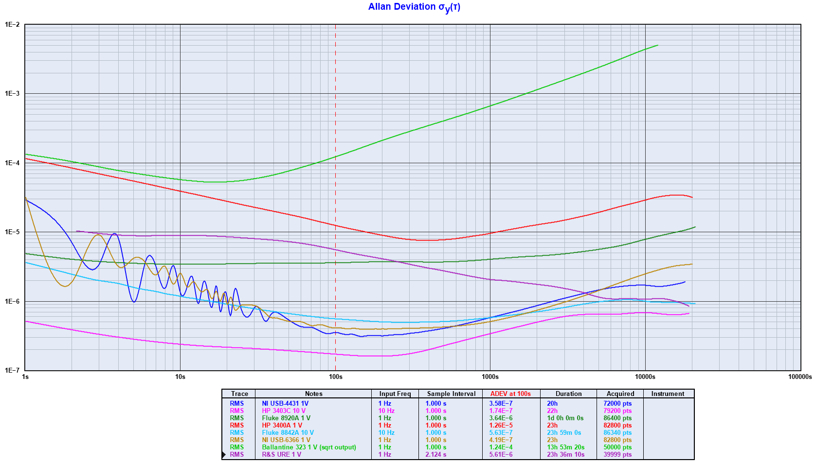
The ADEV of the RMS readings of a selection of RMS instruments, after warm-up. The pleasant surprise is the HP 3403C which appears highly stable once it has reached its working temperature. The stability of the 3403C is better than the number of digits of the display would lead you to believe.
The disappointment is the Ballantine 323, which is plagued by a much too varying output. The R&S URE demonstrates a high degree of stability over long time, but the resolution of its A/D-converter limits the ADEV on the shorter time scale. The DC output option would not help, on the contrary, as the resolution is further reduced by the option's 12-bit A/D-converter. |
Stability
In addition to the bandwidth, the accuracy (proximity to the true value) and precision (stability of measurements) are central performance parameters of an RMS meter. The graph on the left shows the Allan Deviation as a measure of the stability for different RMS meters. The signal source is a Fluke 510A (@ 2.4 kHz) with an inductive voltage divider (Gertsch RT-60 or ESI DT72A) inserted where appropriate. In case a DC output is measured it is done via the Fluke 8842A.
To follow:
|
|
(Picture to be uploaded)
|
Range linearity
Thanks to the accuracy and precision of an inductive voltage divider one may put the RMS meters to the test of their linearity. The figure on the left shows the deviation from the correct reading when going through a range for different RMS voltmeters. If an instruments has an autorange feature, it was disabled during the test. The AC source was a Fluke 510A, running at 2.4 kHz, and the IVD was an ESI DT72A. |
|
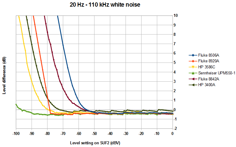
White noise test
The graph to the left shows a comparison between different RMS voltmeters measuring white noise at different levels. The Fluke A55 and the EL-2255 are not included as the test spans over a range of input levels. The graph shows how the error increases as the level is reduced. The source was a Rohde & Schwarz SUF2 Noise Generator, set to 110 kHz noise bandwidth, and with the level varied between 0 and -100 dBV into 75 Ohms. The level of the SUF2 during the test was about 0.4 dB too low due to the level adjustment on the SUF2 front panel. The adjustment was left unchanged during the test to allow comparison. A 75 Ohm feed-through termination was used during the measurements, expect when using the the HP 3586C that was set to 75 Ohm input termination. The ranges for the Sennheiser and the HP 3400A were set so that the largest scale deflection was obtained. The readings from the 3400A were taken from its DC output, measured by Fluke 8842A from which data was captured via GPIB by LabVIEW. The avarage was calculated over 128 readings. Such a setup is required to give reliable readings, especially at the lower end of the scale. Graphs for the 6 MHz and for 50 MHz noise bandwidth settings of the SUF2 are not included here as the flatness of the SUF2 is seriously compromized for these bandwidth settings at low levels. More details are found on the noise generator pages. The jumps around 32 dB and 64 dB are caused by the inaccuracies of the 32 dB and 64 dB attenuator steps of the SUF2. |
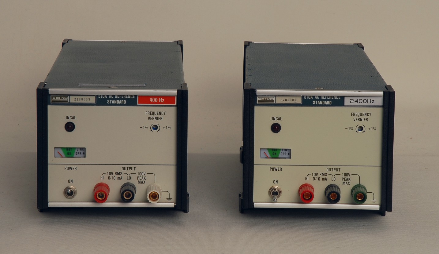
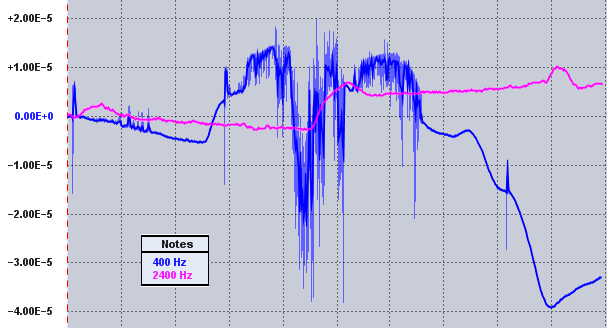
Frequency stability of two different 510A units: The 400 Hz unit before replacement of C6, and the 2400 Hz unit.
Frequency stability after modifications (to be inserted)
Level stability of the same two different 510A units (to be inserted)
|
Fluke 510A AC Reference Standard
This handy unit produces 10 V RMS at a fixed frequency in loads above 1 kOhm for calibration and test. It could be ordered with any frequency between 50 Hz and 100 kHz, with standard options at 50, 60, 400, 1,000, 2,400, 5,000, 19,200 Hz and 100 kHz. The frequency is determined by a plug-in module inside the box, and you may easily modify the frequency, if needed. More up-to-date designs and sources with programmable output level are available, but the 510A remains a reliable workbench tool, and is often spotted on the used market. The picture shows the two different 510A units in my lab, one with 400 Hz output, and another with 2,400 Hz output. Note the slight colour difference of the front plates as well as the different colour of the GND terminal. Older units have a black front plate. At one point the 400 Hz unit started to behave weirdly with irregular frequency and level changes of increasing intensity. Investigations revealed that the ceramic capacitor C6 (47 nF / 25 V) in the feedback loop of the positive supply had turned leaky, thereby resulting in a too low and varying positive rail, and eventually clipping of the output signal. The C6 and the other similar capacitors were replaced with film capacitors, and the 510A was back in shape. To be added: Graph showing the level stability of the two units. |
